La statistica dei rendimenti finanziari e alcune osservazioni empiriche sull'asset allocation - Pagine personali del personale della ...
←
→
Trascrizione del contenuto della pagina
Se il tuo browser non visualizza correttamente la pagina, ti preghiamo di leggere il contenuto della pagina quaggiù

La statistica dei rendimenti
finanziari e alcune osservazioni
 empiriche sull’asset allocation
                         Stefano Marmi
                 http://homepage.sns.it/marmi/
                   Scuola Normale Superiore
 Seminario del 9 giugno 2009 – Corso di Metodi e Modelli per
  l'Analisi Finanziaria – Facoltà di Ingegneria - Università di
                              Siena
Sommario

• Il trionfo degli ottimisti
• Mercati efficienti?
• I fatti stilizzati relativi alle serie storiche dei
  rendimenti
• L‘articolo più scaricato dal SSRN nel 2008
• Il rapporto P/E10 di Shiller
• Alcuni problemi matematici?
                  La statistica dei rendimenti finanziari e alcune
9/06/2009          osservazioni empiriche sull‘asset allocation-     2
                               Stefano Marmi, S.N.S.
Bibliografia
Elroy Dimson, Paul Marsh e Mike Staunton ―Triumph of
  the Optimists‖ (2002, Princeton University Press)
R. Cont ―Empirical properties of asset returns: stylized
  facts and statistical issues‖ Quantitative Finance 1
  (2001) 223–236
M.T. Faber ―A Quantitative Approach to Tactical Asset
  Allocation‖ Journal of Wealth Management 2007
(available at the SSRN preprint database, id1347034)
S.M., A. Risso ―Asset allocation: un esempio di approccio
  quantitativo e tattico‖ Rivista AIAF Ottobre 2008

                   La statistica dei rendimenti finanziari e alcune
9/06/2009           osservazioni empiriche sull‘asset allocation-     3
                                Stefano Marmi, S.N.S.
Stocks, bonds, bills and inflation in
       the UK from 1900 to 2007

              La statistica dei rendimenti finanziari e alcune
9/06/2009      osservazioni empiriche sull‘asset allocation-     4
                           Stefano Marmi, S.N.S.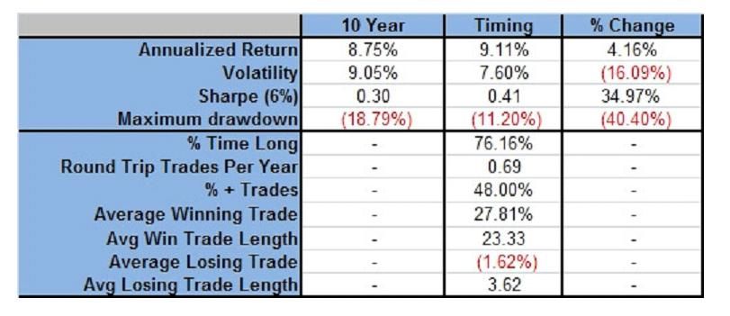
Annualized real (after inflation) returns
   of bonds and stocks: 1900-2007

             La statistica dei rendimenti finanziari e alcune
 9/06/2009    osservazioni empiriche sull‘asset allocation-     5
                          Stefano Marmi, S.N.S.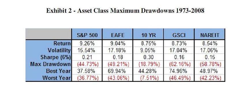
Stock market crashes (before 2008)

             La statistica dei rendimenti finanziari e alcune
9/06/2009     osservazioni empiriche sull‘asset allocation-     6
                          Stefano Marmi, S.N.S.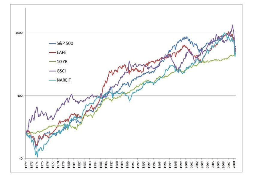
Volatility of stocks

During the period 1900-2007, UK‘s standard deviation of 19.8%
places it alongside the US (20.0%) at the lower end of the risk
spectrum. The highest volatility markets were Germany (32.3%),
Japan (29.8%), and Italy (28.9%), reflecting the impact of wars
and inflation.

                      La statistica dei rendimenti finanziari e alcune
9/06/2009              osservazioni empiriche sull‘asset allocation-     7
                                   Stefano Marmi, S.N.S.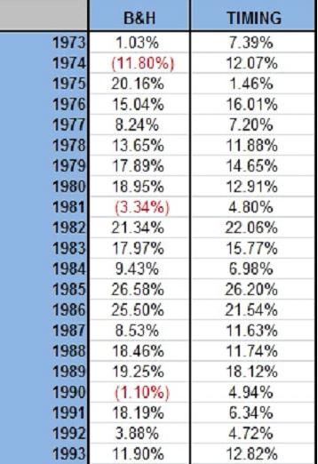
Chicago Board Options Exchange Volatility Index, a popular
measure of the implied volatility of S&P500 index options. A high
value corresponds to a more volatile market and therefore more
costly options, which can be used to defray risk from volatility. If
investors see high risks of a change in prices, they require a greater
premium to insure against such a change by selling options. Often
referred to as the fear index, it represents one measure of the
market's expectation of volatility over the next 30 day period.

                      La statistica dei rendimenti finanziari e alcune
9/06/2009              osservazioni empiriche sull‘asset allocation-     8
                                   Stefano Marmi, S.N.S.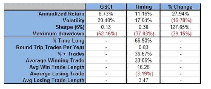
Daily returns of General Motors
                 (1950-2008)

                La statistica dei rendimenti finanziari e alcune
9/06/2009        osservazioni empiriche sull‘asset allocation-     9
                             Stefano Marmi, S.N.S.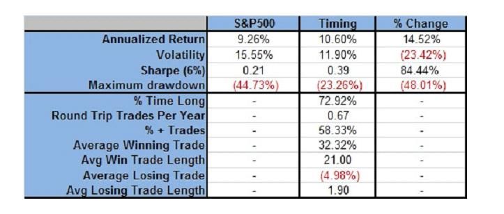
Volatility clustering
Time series plots of returns display an important feature that is
usually called volatility clustering. This empirical phenomenon
was first observed by Mandelbrot (1963), who said of prices that
―large changes tend to be followed by large changes—of either
sign—and small changes tend to be followed by small changes.‖
Volatility clustering describes the general tendency for markets to
have some periods of high volatility and other periods of low
volatility. High volatility produces more dispersion in returns
than low volatility, so that returns are more spread out when
volatility is higher. A high volatility cluster will contain several
large positive returns and several large negative returns, but there
will be few, if any, large returns in a low volatility cluster.
                      La statistica dei rendimenti finanziari e alcune
9/06/2009              osservazioni empiriche sull‘asset allocation-     10
                                   Stefano Marmi, S.N.S.
Daily returns of GM after normalization by
short-term (25 days) volatility
La statistica dei rendimenti finanziari e alcune
9/06/2009 osservazioni empiriche sull‘asset allocation- 11
Stefano Marmi, S.N.S.Stylized facts (R. Cont, Quantitative Finance (2001))
1. Absence of autocorrelations: (linear) autocorrelations of asset returns
are often insignificant, except for very small intraday time scales (≈ 20
minutes) for which microstructure effects come into play.
2. Heavy tails: the (unconditional) distribution of returns seems to
display a power-law or Pareto-like tail, with a tail index which is finite,
higher than two and less than five for most data sets studied. In
particular this excludes stable laws with infinite variance and the
normal distribution. However the precise form of the tails is difficult to
determine.
3. Gain/loss asymmetry: one observes large drawdowns in stock prices
and stock index values but not equally large upward movements
La statistica dei rendimenti finanziari e alcune
9/06/2009 osservazioni empiriche sull‘asset allocation- 12
Stefano Marmi, S.N.S.Do daily returns follow a
normal distribution? Observed Theoretical
Class Frequency Frequency
x< -0.05 67 0.093902
Mean 00204
-0.05Distribution of returns of DJIA stocks: from
―Foundations of Finance‖, Fama (1976)
La statistica dei rendimenti finanziari e alcune
9/06/2009 osservazioni empiriche sull‘asset allocation- 14
Stefano Marmi, S.N.S.La statistica dei rendimenti finanziari e alcune
9/06/2009 osservazioni empiriche sull‘asset allocation- 15
Stefano Marmi, S.N.S.Theoretical and observed frequency of outliers
in the history of 15 stockmarkets
La statistica dei rendimenti finanziari e alcune
Estrada, Javier: Black Swans and Market Timing:
9/06/2009 osservazioni
How Not toempiriche
Generatesull‘asset
Alpha. allocation- 16
Available at SSRN: http://ssrn.com/abstract=1032962 Stefano Marmi, S.N.S.Stylized facts (R. Cont, Quantitative Finance (2001))
4. Aggregational Gaussianity: as one increases the time scale Δt over
which returns are calculated, their distribution looks more and more
like a normal distribution. In particular, the shape of the distribution is
not the same at different time scales.
5. Intermittency: returns display, at any time scale, a high degree of
variability. This is quantified by the presence of irregular bursts in time
series of awide variety of volatility estimators.
6. Volatility clustering: different measures of volatility display a
positive autocorrelation over several days, which quantifies the fact that
high-volatility events tend to cluster in time.
7. Conditional heavy tails: even after correcting returns for volatility
clustering (e.g. via GARCH-type models), the residual time series still
exhibit heavy tails. However, the tails are less heavy than in the
unconditional distribution of returns.
La statistica dei rendimenti finanziari e alcune
9/06/2009 osservazioni empiriche sull‘asset allocation- 17
Stefano Marmi, S.N.S.Volatility clustering and leverage effect
160
140
120
100
80
numero giorni >1%
numero giorniStylized facts (R. Cont, Quantitative Finance (2001))
8. Slow decay of autocorrelation in absolute returns: the
autocorrelation function of absolute returns decays slowly as a
function of the time lag, roughly as a power law with an exponent
β ∈ [0.2, 0.4]. This is sometimes interpreted as a sign of long-
range dependence.
9. Leverage effect: most measures of volatility of an asset are
negatively correlated with the returns of that asset.
10. Volume/volatility correlation: trading volume is correlated
with all measures of volatility.
11. Asymmetry in time scales: coarse-grained measures of
volatility predict fine-scale volatility better than the other way
round.
La statistica dei rendimenti finanziari e alcune
9/06/2009 osservazioni empiriche sull‘asset allocation- 19
Stefano Marmi, S.N.S.Autocorreletion of daily returns and of their absolute values. The black
line is the best power law fit of the absolute values autocorrelations
0.4
Index: DJIA (1885-2008)
0.35
0.3
0.25
y = 0.3697x -0.225
0.2 R² = 0.935
0.15
0.1
0.05
0
0 10 20 30 40 50 60 70 80 90 100
-0.05
La statistica dei rendimenti finanziari e alcune
9/06/2009 osservazioni empiriche sull‘asset allocation- 20
-0.1 Stefano Marmi, S.N.S.Cos’è un mercato efficiente (borsa,
sala corse, ecc)?
Un mercato è efficiente quando è efficiente nell‘elaborazione delle
informazioni: i prezzi dei beni (azioni, quote del bookmaker,
obbligazioni, materie prime, ecc) osservati in ogni istante di tempo
sono il risultato di una valutazione ―corretta‖ di tutta l‘informazione
disponibile al momento. I prezzi ―riflettono pienamente‖ tutta
l‘informazione disponibile, sono sempre ―fair‖, cioè buone indicazioni
dei valori in gioco.
Bachelier (1900) scrive che ―Les influences qui déterminent les
mouvements de la Bourse sont innombrables, des événements passés,
actuels ou même escomptables, ne présentant souvent aucun rapport
apparent avec ses variations, se répercutent sur son cours‖
…‖Si le marché, en effet, ne prévoit pas les mouvements, il les
considère comme étant plus ou moins probables, et cette probabilité
peut s‘évaluer mathématiquement.‖
La statistica dei rendimenti finanziari e alcune
9/06/2009 osservazioni empiriche sull‘asset allocation- 21
Stefano Marmi, S.N.S.Efficienza forte e debole
Un mercato è efficiente rispetto a un ―insieme‖ di informazioni
Θt se i prezzi non cambierebbero rivelando queste informazioni a
tutti gli agenti → non è possibile fare profitti utilizzando Θt per il
trading
La forma debole dell‘ipotesi dei mercati efficienti richiede che i
prezzi rispecchino pienamente l‘informazione implicita nella
successione dei prezzi passati. La forma semi-forte asserisce che i
prezzi rispecchiano tutta l‘informazione pubblicamente
disponibile mentre nella forma forte i prezzi riflettono anche
l‘informazione non pubblicamente disponibile ma conosciuta da
almeno un agente.
La statistica dei rendimenti finanziari e alcune
9/06/2009 osservazioni empiriche sull‘asset allocation- 22
Stefano Marmi, S.N.S.―However, we might define an efficient
market as one in which price is within a
factor of 2 of value, i.e. the price is
more than half of value and less than
twice value. The factor of 2 is arbitrary,
of course. Intuitively, though, it seems
reasonable to me, in the light of sources
of uncertainty about value and the
strength of the forces tending to cause
price to return to value. By this
definition, I think almost all markets are
efficient almost all of the time. ‗Almost
all‘ means at least 90% ―
Fischer Sheffey Black (January F. Black, Noise, Journal of Finance (1986)
11, 1938 – August 30, 1995)
p. 533.
La statistica dei rendimenti finanziari e alcune
9/06/2009 osservazioni empiriche sull‘asset allocation- 23
Stefano Marmi, S.N.S.La statistica dei rendimenti finanziari e alcune
9/06/2009 osservazioni empiriche sull‘asset allocation- 24
Stefano Marmi, S.N.S.Critiche all’ipotesi dei mercati
efficienti
Grossman and Stiglitz (―On the Impossibility of Informatioally Efficient Markets, American
Economic Review, 70, 393-408, 1980) argue that perfectly informationally efficient markets
are an impossibility. Roughly speaking the idea is more or less that if markets were perfectly
efficient, there would be no profit to gathering information, in which case (in an equilibrium
world) there would be little reason to trade and markets would eventually collapse.
Alternatively, the degree of market inefficiency determines the effort investors are willing to
expend to gather and trade on information, hence a non-degenerate market equilibrium will arise
only when there are sufficient profit opportunities, i.e., inefficiencies, to compensate investors for
the costs of trading and information-gathering. The profits earned by these attentive
investors may be viewed as ―economic rents‖ that accrue to those willing to engage in such
activities. Who are the providers of these rents? Black (1986) gave us a provocative answer:
―noise traders‖, individuals who trade on what they consider to be information but which is, in
fact, merely noise.
(From A. Lo, The Adaptive Market Hypothesis, Journal of Portfolio Management 2004)
La statistica dei rendimenti finanziari e alcune
9/06/2009 osservazioni empiriche sull‘asset allocation- 25
Stefano Marmi, S.N.S.La difesa:
Can Predicable Patterns in Market
Returns be Exploited Using Real Money?
Not likely.
La statistica dei rendimenti finanziari e alcune
9/06/2009 osservazioni empiriche sull‘asset allocation- 26
Stefano Marmi, S.N.S.Benjamin Graham (5/8/1894-9/21/1976)
was an American economist and professional investor. First proponent
of value investing, an investment approach he began teaching at Columbia
Business School in 1928 and subsequently refined with David Dodd
through various editions of their famous book Security Analysis. His most
famous disciples is Warren Buffet, who credits Graham as grounding him
with a sound intellectual investment framework. Graham recommended
that investors spend time and effort to analyze the financial state of
companies. When a company is available on the market at a price which is
at a discount to its fair value, a margin of safety exists, which makes it
suitable for investment.
Graham's favorite allegory is that of Mr. Market, a fellow who turns up
every day at the stock holder's door offering to buy or sell his shares at
a different price. Often, the price quoted by Mr. Market seems
plausible, but often it is ridiculous. The investor is free to either agree
with his quoted price and trade with him, or to ignore him completely.
Mr. Market doesn't mind this, and will be back the following day to
quote another price. The point is that the investor should not regard the
whims of Mr. Market as determining the value of the shares that the
investor owns. He should profit from market folly rather than
participate in it. The investor is best off concentrating on the real life
performance of his companies and receiving dividends, rather than
La statistica dei rendimenti finanziari e alcune
being9/06/2009
too concerned with Mr. Market's oftenempiriche
osservazioni irrational behavior.
sull‘asset allocation- 27
Stefano Marmi, S.N.S.Charles Henry Dow (b.11/6/1851, d.12/4/1902)
cofounded Dow Jones & Company with E. Jones and C.
Bergstesser. Dow also founded The Wall Street Journal,
which became one of the most respected financial
publications in the world. He also invented the famous Dow
Jones Industrial Average as part of his research into market
movements. Furthermore he developed a series of principles
for understanding and analyzing market behavior which
later became known as Dow theory, the groundwork
for technical analysis.
Dow published the Wall Street Journal beginning in 1889. He wrote during a period
of generally rising stock prices from the depression lows in the 1870s to the then all
time high in 1901. During that period Dow formulated his theory of the stock
market. It consisted of two important components: the cyclical nature of the market
and in the longer cycle, the ―third wave‖, the need for confirmation between
economically different sectors, specifically the industrials and the railroads.
“Nothing is more certain that the market has three well-defined movements which fit
into each other. The first is the variation due to local causes and the balance of
buying and selling at that particular time. The secondary movement covers a period
ranging from 10 days to 60 days, averaging probably between 30 and 40 days. The
third movement is the great Laswing
9/06/2009
statisticacovering
dei rendimentifrom four
finanziari
osservazioni empiriche sull‘asset allocation-
to six years.”
e alcune
28
Stefano Marmi, S.N.S.Analisi tecnica e analisi fondamentale
Fundamental analysis maintains that markets may misprice a security in
the short run but that the "correct" price will eventually be reached.
Analyzing financial statements, management and competitive
advantages, one can accurately estimate a ―fair value‖ for the stock.
Profits can be made by trading the mispriced security and then waiting
for the market to recognize its "mistake" and reprice the security.
Technical analysis maintains that all information is reflected already in
the stock price, so fundamental analysis is a waste of time. Trends 'are
your friend' and sentiment changes predate and predict trend changes.
Investors' emotional responses to price movements lead to recognizable
price chart patterns. Technical analysis does not care what the 'value' of a
stock is. Their price predictions are only extrapolations from historical
price patterns.
La statistica dei rendimenti finanziari e alcune
9/06/2009 osservazioni empiriche sull‘asset allocation- 29
Stefano Marmi, S.N.S.If the markets is efficient the market price of a stock is the best
possible estimate of its value. Fundamental analysis is reduced
to a process which can verify that the market estimate of the
value of the stock is correct. If the market is not perfectly
efficient, the price of a stock can differ from its value quite
considerably and fundamental analysis may be used profitably.
The efficient market hypothesis does not require that the price is
always equal to the value: it is sufficient that valuation mistakes
do not obey to any logic, so that they are completely random
and uncorrelated so that the probability that a given stock is
under/overvalued is the same at all times.
But…what should be the value of a stock?
La statistica dei rendimenti finanziari e alcune
9/06/2009 osservazioni empiriche sull‘asset allocation- 30
Stefano Marmi, S.N.S.Formulazione debole dell’IME
In weak-form efficiency excess returns cannot be made by using
investment strategies based on historical prices or other historical
financial data: for example it will not be possible to make excess
returns by using methods such as technical analysis. A trading
strategy incorporating historical data, such as price and volume
information, will not systematically outperform a buy-and-hold
strategy. It is often said that current prices accurately incorporate
all historical information, and that current prices are the best
estimate of the value of the investment. Prices will respond to
news, but if this news is random then price changes will also be
random. Technical analysis will not be profitable.
La statistica dei rendimenti finanziari e alcune
9/06/2009 osservazioni empiriche sull‘asset allocation- 31
Stefano Marmi, S.N.S.Le idee alla base dell’analisi tecnica
- I prezzi sono unicamente determinati dalla domanda e
dall‘offerta
- La domanda e l‘offerta sono governate da fattori razionali e
irrazionali. Il mercato valuta tutti questi fattori continuamente.
- I prezzi delle azioni e degli asset tendono a seguire dei trend
che hanno una durata apprezzabile nel tempo
- I cambiamenti dei trend sono dovuti a spostamenti della
domanda e dell‘offerta, così come a cambiamenti del quadro
macroeconomico. I cambiamenti possono essere rilevati dalla
dinamica dei prezzi di mercato
La statistica dei rendimenti finanziari e alcune
9/06/2009 osservazioni empiriche sull‘asset allocation- 32
Stefano Marmi, S.N.S.Journal of Wealth
Management (2007) and
2009 update available at
the SSRN preprint
database, id1347034
This article examines a very simple quantitative market-timing model. This trend
following model is examined in-sample on the U.S. stock market since 1900 before
out-of-sample testing across more than twenty other markets. The attempt is not to
build an optimization model (indeed, the chosen model is decidedly sub-optimal, as
evidenced later in the article), but to build a simple trading model that works in the
vast majority of markets. The results suggest that a market timing solution is
a risk-reduction technique rather than a return-enhancing one. The approach is then
examined in an allocation framework since 1972, including such diverse asset
classes as the Standard and Poor‘s 500 Index (S&P 500), Morgan Stanley Capital
International Developed Markets Index (MSCI EAFE), Goldman Sachs Commodity
Index (GSCI), National Association of Real Estate Investment Trusts Index
(NAREIT), and United States Government 10-Year Treasury Bonds. The empirical
results are equity-like returns with bond-like volatility and drawdown, and over
thirty consecutive years of positive returns.
La statistica dei rendimenti finanziari e alcune
9/06/2009 osservazioni empiriche sull‘asset allocation- 33
Stefano Marmi, S.N.S.BUY RULE
Buy when monthly price
> 10-month SMA.
SELL RULE
Sell and move to cash
when monthly price <
10-month SMA.
1. All entry and exit
prices are on the day
of the signal at the
close.
2. All data series are total
return series including
dividends, updated
monthly.
3. Cash returns are
estimated with 90-day
commercial paper.
4. Taxes, commissions,
and slippage are
excluded .
La statistica dei rendimenti finanziari e alcune
9/06/2009 osservazioni empiriche sull‘asset allocation- 34
Stefano Marmi, S.N.S.Efficienza forte e semi-forte
In the semi-strong form of the EMH a trading strategy
incorporating current publicly available fundamental information
(such as financial statements) and historical price information
will not systematically outperform a buy-and-hold strategy. Share
prices adjust instantaneously to publicly available new
information, and no excess returns can be earned by using that
information. Fundamental analysis will not be profitable.
In strong-form efficiency share prices reflect all information,
public and private, fundamental and historical, and no one can
earn excess returns. Inside information will not be profitable.
La statistica dei rendimenti finanziari e alcune
9/06/2009 osservazioni empiriche sull‘asset allocation- 35
Stefano Marmi, S.N.S.50 20
45 18
2000
40 16
35 1981 14
Long-Term Interest Rates
30 12
Price-Earnings Ratio
25 10
1901 1966
20 Price-Earnings Ratio 8
15 6
10 1921 15.3 4
5 2
Long-Term Interest Rates
0 0
1860 1880 1900 1920 1940 1960 1980 2000 2020
Year
Robert Shiller's plot of the S&P Composite Real Price-Earnings Ratio and Interest
Rates (1871–december 2008), from Irrational Exuberance, 2d ed.[1] In the preface
to this edition, Shiller warns that "[t]he stock market has not come down to
historical levels: the price-earnings ratio as I define it in this book is still, at this
writing [2005], in the mid-20s, far higher than the historical average. … People still
place too much confidence in the markets and have too strong a belief that paying
attention
9/06/2009
to the gyrations inLaosservazioni
their investments
statistica will someday
dei rendimenti finanziari e alcune
empiriche sull‘asset allocation-
make them rich, and
36
so
they do not make conservative preparations Stefano Marmi, for
S.N.S.possible bad outcomes."P/E ratios as a predictor of long term
U.S. stocks returns
Price-Earnings ratios as a predictor of twenty-year returns based upon the plot
by Robert Shiller (Figure 10.1 Irrational Exuberance, Princeton University
Press.). The horizontal axis shows the real price/earnings ratio of the S&P500
index (inflation adjusted price divided by the prior ten-year mean of inflation-
adjusted earnings). The vertical axis shows the geometric average real annual
return on investing in the S&P500 index, reinvesting dividends, and selling ten
or twenty years later. Data from different ten/twenty year periods is color-
coded as shown in the key. According to Shiller these plots "confirms that
long-term investors—investors who commit their money to an investment for
ten full years—did do well when prices were low relative to earnings at the
beginning of the ten years. Long-term investors would be well advised,
individually, to lower their exposure to the stock market when it is high, as it
has been recently, and get into the market when it is low."
La statistica dei rendimenti finanziari e alcune
9/06/2009 osservazioni empiriche sull‘asset allocation- 37
Stefano Marmi, S.N.S.S&P ≈700 (febbraio 2009)
E(10-year) ≈ 56
P/E(10.year) ≈ 12.5
La statistica dei rendimenti finanziari e alcune
9/06/2009 osservazioni empiriche sull‘asset allocation- 38
Stefano Marmi, S.N.S.S&P ≈700 (febbraio 2009)
E(10-year) ≈ 56
P/E(10.year) ≈ 12.5
La statistica dei rendimenti finanziari e alcune
9/06/2009 osservazioni empiriche sull‘asset allocation- 39
Stefano Marmi, S.N.S.Alcune analisi statistiche tuttavia indicano come, almeno in certi periodi, le
variazioni di prezzo settimanali e mensili non siano completamente
indipendenti dal passato e alcuni semplici indicatori fondamentali o tecnici (i
multipli e il momento, tanto per citarne due dei più importanti) possano avere
una qualche capacità di predire l‘andamento futuro dei prezzi. Così, da almeno
venti anni, la letteratura accademica si interroga sulla significatività (statistica
ed economica) delle numerose anomalie riscontrate nelle serie storiche dei
rendimenti azionari..È oggetto di controversia il fatto che gli investitori possano
farne uso per ottenere dei rendimenti superiori ai benchmark. Gli investitori
interessati a strategie di investimento che cerchino di utilizzare queste anomalie
devono ricordare che nulla ci assicura che continueranno a prodursi in futuro:
come sempre, come ben sappiamo, ―i rendimenti passati non sono garanzia di
rendimenti futuri‖ … Le anomalie possono scomparire perché, prive di una
base economico-finanziaria, sono semplicemente frutto del data mining, oppure
essere cancellate dall‘arbitraggio compiuto da investitori (hedge funds, ad
esempio) che prendono ad utilizzarle come strategie d‘investimento.
La statistica dei rendimenti finanziari e alcune
9/06/2009 osservazioni empiriche sull‘asset allocation- 40
Stefano Marmi, S.N.S.Fisher Black warning concerning anomalies: Most so-called anomalies don't
seem anomalous to me at all. They seem like nuggets from a gold mine, found
by one of the thousands of miners all over the world. Si veda anche l‘articolo
―Noise‖, Journal of Finance vol 41, no. 3, 529-543 (1993)
The most famous ―anomaly‖, very often recommended as a long-term
investment strategy, corresponds to the so-called value investing. There is a
quite convincing statistical evidence that investors tend to overvalue future
growth prerspectives in companies with a past record with high earnings
growth rates and to underestimate the future perspectives of value stocks, i.e.
stocks with low multiples (P/E price to earnings, P/BV price to book value,
P/D price to dividend, etc. ) i.e. multiples which are below market and7Or
sector averages
Capaul, C., I. Rowley, W.F. Sharpe ―International Value and Growth Stock
Returns.‖ Financial Analysts Journal, vol. 49, no. 1 (January/February
1993):27-36
Fama, E.F, e K.R. French ―Value versus Growth: The International
Evidence.‖ Journal of Finance, vol. 53, no. 6(December 1998):1975-1999.
La statistica dei rendimenti finanziari e alcune
9/06/2009 osservazioni empiriche sull‘asset allocation- 41
Stefano Marmi, S.N.S.Elroy Dimson, Paul Marsh e Mike Staunton (Triumph of the Optimists (2002,
Princeton University Press) : analisi dei rendimenti di azioni e obbligazioni e
dell‘inflazione in 16 paesi dal 1900 al 2000.
il rendimento annuo composto nominale (al lordo dell‘inflazione e trascurando
le tasse e i costi di negoziazione) delle azioni è stato
USA 10.1% = 5.4% capital gain + 4.7% dividendi reinvestiti.
UK 10.1% = 5.1% capital gain + 5% dividendi reinvestiti
Più è lungo l‘orizzonte temporale di un investitore, più importante diventa il
rendimento dovuto ai dividendi: su 100 anni l‘effetto moltiplicatore dei
dividendi corrisponde a un fattore 85 nel caso americano, 109 nel caso inglese.
Limitandosi al mercato USA, in un editoriale del Financial Analysts Journal nel
2003 Robert Arnott ha analizzato i rendimenti azionari dal 1802 al 2002. Il
rendimento annualizzato delle azioni è circa il 7.9% scomponibile in 5% di
rendimento dai dividendi e dal loro reinvestimento, 0.8% dall‘aumento dei
dividendi reali (al netto dell‘inflazione) 1.5% dall‘inflazione, 0.6% dall‘aumento
secolare dei multipli azionari (in questo caso l‘inverso del rapporto D/P):
―Dividends not only dwarf inflation, growth, and changing valuation levels
individually, but they also dwarf the combined importance of inflation, growth,
and changing valuation levels.‖
La statistica dei rendimenti finanziari e alcune
9/06/2009 osservazioni empiriche sull‘asset allocation- 42
Stefano Marmi, S.N.S.I portafogli ad alto rapporto dividendo/prezzo
Già nel 1920 Charles Dow raccomandava l‘uso del rapporto dividendo/prezzo per il mercato come indicatore dei
rendimenti futuri. In questo caso il rapporto è ottenuto dividendo l‘ammontare complessivo di tutti i dividendi pagati
dalle azioni quotate per la capitalizzazione complessiva del mercato. Molti anni dopo Fama e French (1988) mostrarono
come il rapporto dividendo/prezzo complessivo del mercato statunitense fosse un attendibile indicatore dei rendimenti
futuri su una scala temporale di 1-4 anni. Le azioni che pagano alti dividendi in modo sostenibile (cioè con un payout
ratio=dividendo/utile non troppo alto) sembrano competere con le obbligazioni in modo soddisfacente e dimostrano di
avere una discreta resistenza durante le fasi di mercato ―orso‖. Il reinvestimento dei dividendi sembra inoltre diminuire
sensibilmente il tempo necessario per recuperare le perdite.
L‘analisi statistica delle serie storiche dei rendimenti azionari suggerisce che i portafogli costituiti dai titoli con il più alto
rapporto dividendo/prezzo (D/P) producano rendimenti superiori rispetto ai portafogli costruiti con titoli con rapporto
più basso. Kenneth French ha costruito dei portafogli azionari suddividendo tutte le azioni che pagano un dividendo in
due classi: le azioni ad alto rapporto D/P (corrispondenti al top 30%) e a basso rapporto D/P (corrispondenti al bottom
30%) e ribilanciati annualmente e pesi proporzionali alla capitalizzazione di borsa. Per confronto il rendimento del
mercato si ottiene considerando tutte le azioni considerate più quelle che non pagano necessariamente un dividendo. I
risultati nel periodo 1975-2006 per i mercati italiano, francese, tedesco, inglese, giapponese e cinese (Hong Kong) sono
raccolti nella Tavola 1. Il portafoglio ad alto rapporto D/P ha avuto rendimenti superiori al mercato in tutti e sei i casi,
mediamente del 3%, con una volatilità (calcolata mediante i rendimenti annuali) inferiore nella metà dei casi, e appena
superiore nei rimanenti tre casi. In cinque casi su sei il portafoglio ad alto dividendo ha anche registrato la perdita
inferiore nell‘anno peggiore dei 32 anni presi in considerazione.
Triumph of the Optimists: 101 Years of Global Investment Returns (2002) Princeton University Press.
Dividends and the Three Dwarfs, “Editor’s Corner”, Robert D. Arnott, Financial Analysts Journal, 2003, p. 6. L‘analisi
di Arnott si basa sugli studi di G. William G. Schwert, (―Indexes of United States Stock Prices from 1802 to 1987.‖
Journal of Business, vol. 63, no. 3 (July):399–426 (1990)) e di Jeremy J. Siegel (Stocks for the Long Run. 3rd ed. New
York:
McGraw Hill, 2002)
―I dividendi non solamente giganteggiano se confrontati all‘inflazione, alla crescita o al cambiamento dei livelli delle
valutazioni, ma anche rispetto all‘effetto combinato dell‘inflazione, della crescita e del cambiamento dei livelli delle
valutazioni‖.
Si veda, ad esempio, la discussione in Jeremy J. Siegel: ―The Future for Investors‖ Crown Business, New York (2005),
Chapter 10. Siegel ha definito ―bear market protector‖ e ―return accelerator‖ l‘effetto che il reinvestimento dei dividendi
ha durante i periodi di diminuzione degli indici azionari, diminuendo a volte in modo sostanziale il tempo necessario per
recuperare le perdite subite.
La statistica dei rendimenti finanziari e alcune
9/06/2009 osservazioni empiriche sull‘asset allocation- 43
Stefano Marmi, S.N.S.Returns of portfolios constructed selecting the top 30% and bottom 30% D/P
ratios (1975-2006) (portfolios constructed by K. French, cfr.
http://mba.tuck.dartmouth.edu/pages/faculty/ken.french/index.html)
UK HK JAP
Market High D/P Low D/P market High D/P Low D/P market High D/P Low D/P
average 19.6 21.2 17.4 24.6 28.8 26.0 9.7 13.4 6.8
Standard
dev. 27.1 27.9 26.5 36.9 32.4 40.6 22.6 22.8 25.4
min ret -22.0 -21.6 -26.8 -39.4 -33.3 -49.4 -38.9 -39.1 -41.7
max ret 145.3 141.5 131.3 121.0 112.0 116.2 62.4 78.2 85.3
IT FR GER
market High D/P Low D/P market High D/P Low D/P market High D/P Low D/P
average 18.0 20.1 16.5 17.5 22.2 13.2 13.6 15.6 12.5
Standard
dev. 33.2 33.9 38.9 25.6 23.9 27.7 24.3 22.4 27.8
min ret -31.1 -29.4 -31.5 -29.3 -21.9 -30.2 -41.0 -35.0 -51.2
max ret 111.3 109.4 123.3 62.5 65.3 65.5 76.9 65.4 93.0
La statistica dei rendimenti finanziari e alcune
9/06/2009 osservazioni empiriche sull‘asset allocation- 44
Stefano Marmi, S.N.S.L’articolo più scaricato dal SSRN
nel 2008 (beh per essere sinceri è il terzo in classifica)
La statistica dei rendimenti finanziari e alcune
9/06/2009 osservazioni empiriche sull‘asset allocation- 45
Stefano Marmi, S.N.S.La statistica dei rendimenti finanziari e alcune
9/06/2009 osservazioni empiriche sull‘asset allocation- 46
Stefano Marmi, S.N.S.La statistica dei rendimenti finanziari e alcune
9/06/2009 osservazioni empiriche sull‘asset allocation- 47
Stefano Marmi, S.N.S.Cinque assets + liquidità
La statistica dei rendimenti finanziari e alcune
9/06/2009 osservazioni empiriche sull‘asset allocation- 48
Stefano Marmi, S.N.S.La statistica dei rendimenti finanziari e alcune
9/06/2009 osservazioni empiriche sull‘asset allocation- 49
Stefano Marmi, S.N.S.L’esempio di Malkiel (riduzione
del rischio via diversificazione)
Ombrelli S.p.A. Ombrelloni
S.p.A.
Stagione +50% -25%
piovosa
Stagione -25% +50%
soleggiata
La statistica dei rendimenti finanziari e
9/06/2009 alcune osservazioni empiriche sull‘asset 50
allocation- Stefano Marmi, S.N.S.Portafoglio 50/50 in entrambe le
società
• Rendimento =
– Pioggia : (0.5) (0.50) + (0.5)(-0.25) = 12.5%
– Sole: (0.5) (-0.25) + (0.5)(0.50) = 12.5%
– = 12.5% sia che piova sia che ci sia il sole
• Il rischio è nullo
• La bellezza della diversificazione
• Il modo più semplice di gestire il rischio
• Funziona particolarmente bene perchè gli asset
sono anticorrelati
La statistica dei rendimenti finanziari e alcune
9/06/2009 osservazioni empiriche sull‘asset allocation- 51
Stefano Marmi, S.N.S.L’origine del miracolo
• I rendimenti degli asset sono perfettamente
―anticorrelati‖
• Entrambi gli asset hanno un rendimento atteso
positivo (=12.5%)
• Non è indispensabile che entrambe le
condizioni siano verificate in ogni istante
La statistica dei rendimenti finanziari e alcune
9/06/2009 osservazioni empiriche sull‘asset allocation- 52
Stefano Marmi, S.N.S.La statistica dei rendimenti finanziari e alcune
9/06/2009 osservazioni empiriche sull‘asset allocation- 53
Stefano Marmi, S.N.S.Timing
BUY RULE
• Buy when monthly price > 10-month SMA.
SELL RULE
• Sell and move to cash when monthly price < 10-month SMA.
1. All entry and exit prices are on the day of the signal at the
close. The model is only updated once a month on the last day
of the month. Price fluctuations during the rest of the month are
ignored.
2. All data series are total return series including dividends,
updated monthly.
3. Cash returns are estimated with 90-day Treasury bills
4. Taxes, commissions,
9/06/2009
and deislippage
La statistica are eexcluded
rendimenti finanziari alcune
osservazioni empiriche sull‘asset allocation- 54
Stefano Marmi, S.N.S.La statistica dei rendimenti finanziari e alcune
9/06/2009 osservazioni empiriche sull‘asset allocation- 55
Stefano Marmi, S.N.S.La statistica dei rendimenti finanziari e alcune
9/06/2009 osservazioni empiriche sull‘asset allocation- 56
Stefano Marmi, S.N.S.La statistica dei rendimenti finanziari e alcune
9/06/2009 osservazioni empiriche sull‘asset allocation- 57
Stefano Marmi, S.N.S.35 anni di profitti
La statistica dei rendimenti finanziari e alcune
9/06/2009 osservazioni empiriche sull‘asset allocation- 58
Stefano Marmi, S.N.S.Puoi anche leggere