POLITECNICO DI TORINO - Corso di Laurea Magistrale in Ingegneria Aerospaziale - Geometrically Nonlinear Analysis of Axial Rotors - Webthesis

POLITECNICO DI TORINO
 Corso di Laurea Magistrale in Ingegneria Aerospaziale

 TESI DI LAUREA MAGISTRALE

Geometrically Nonlinear Analysis of Axial Rotors

Relatori
Prof. Erasmo Carrera
Prof. Matteo Filippi

 Candidato:
 Alessandro Maturi

 Luglio 2021

2 Alessandro Maturi - s255506

 Tesi di Laurea Magistrale – AA 2020-2021

Alessandro Maturi - s255506 3

 “La montagna più alta rimane
 sempre dentro di noi”

 Walter Bonatti

Tesi di Laurea Magistrale – AA 2020-2021

4 Alessandro Maturi - s255506

 Tesi di Laurea Magistrale – AA 2020-2021

Alessandro Maturi - s255506 5

Ringraziamenti

Voglio dedicare questo spazio iniziale a tutti coloro che, con il loro supporto, mi hanno aiutato in
questo lungo e meraviglioso percorso di crescita personale e di approfondimento delle
conoscenze acquisite durante i miei anni universitari.

Un enorme ringraziamento va innanzitutto ai miei genitori, fonte di sostegno e di coraggio, per
avermi trasmesso la passione per lo studio e la forza di volontà necessaria per raggiungere
questo traguardo. Grazie per tutti i consigli e in particolar modo per le esperienze ed i viaggi che
mi avete permesso di vivere insieme a voi fin da bambino: anche se è impossibile ricordare tutti
quei momenti, sono assolutamente certo che essi siano stati fondamentali per la determinazione
del mio carattere e del mio modo di pensare. Dal picco del Preikestolen in Norvegia, passando
attraverso i viaggi in camper in Europa fino ai grattacieli di New York, avete dato a me e a mia
sorella una diversa prospettiva sul mondo e gli strumenti per approfondire, forse anche troppo,
ogni situazione. Senza tale spinta propulsiva non sarei qui oggi a dedicarvi la gioia di questo
momento.

Un sentito grazie anche a mia sorella Laura, per i nostri dibattiti e scambi di idee portati avanti
in questo anno di Covid, durante il quale, dopo molto tempo, siamo tornati a vivere nella stessa
casa: continua con la tua determinazione verso il tuo prossimo, vicino obiettivo.

Un ringraziamento a tutti gli amici di spirito e compagni di avventure di Fiavè, di Burro, del
Bleggio e di Torino: i momenti di svago e di montagna passati con voi durante i weekend e in
estate sono stati fondamentali per ricaricarsi tra le sessioni di esami.

Per ultimi, ma non meno importanti, voglio qui ringraziare i professori Carrera e Filippi, relatori
di questo lavoro di tesi. Il loro supporto e disponibilità nel fornire consigli sono stati cruciali per
la stesura dell’elaborato finale.

 Tesi di Laurea Magistrale – AA 2020-2021

6 Alessandro Maturi - s255506

 Acknowledgements

 I’d like to dedicate this initial space to all those who, with their support, have helped me in this
 long and wonderful journey of personal growth and deepening of the knowledge acquired during
 my university years.

 First of all, a huge thanks goes to my parents, a source of support and courage, for giving me the
 passion for studying and the willpower necessary to reach this goal. Thanks for all the advice
 and especially for the experiences and travels that you have allowed me to live with you since I
 was a child: even if it is impossible to remember all those moments, I am absolutely sure that
 they were fundamental for the determination of my character and my way of thinking. From the
 peak of Preikestolen in Norway, passing through motorhome trips in Europe to the skyscrapers
 of New York, you have given my sister and me a different perspective on the world and the tools
 to explore, perhaps too much, every situation. Without this driving force I would not be here
 today to dedicate the joy of this moment to you.

 A heartfelt thanks also to my sister Laura, for our debates and exchanges of ideas carried out in
 this year of Covid, during which, after a long time, we have returned to live in the same house:
 continue with your determination towards your next, near goal.

 Thanks to all the friends and adventure mates of Fiavè, Burro, Bleggio and Turin: the moments
 of leisure spent with you and in the mountains during the weekends and in the summer were
 fundamental to recharge between the exam sessions.

 Last but not least, I want here to thank professors Carrera and Filippi, supervisors of this thesis
 work. Their support and availability in providing advice were crucial for the drafting of the final
 thesis paper.

 Tesi di Laurea Magistrale – AA 2020-2021

Alessandro Maturi - s255506 7

Sommario
Questo lavoro di tesi è focalizzato sull’analisi di sistemi rotanti complessi, soggetti a
condizioni operative plausibili nella realtà pratica delle applicazioni aeronautiche. Vengono
valutati gli effetti rotordinamici introdotti dalla forza centrifuga; in particolare, l’analisi verrà
portata avanti considerando dischi con spessore costante e variabile, che vengono assunti
incastrati all’hub o supportati da un albero deformabile e quindi flessibile, non rigido.

I contributi del pre-stress sono stati ottenuti attraverso l’integrazione di uno stato di tensione
tridimensionale, che viene generato prevalentemente dai carichi centrifughi, moltiplicati dai
termini non lineari del campo di deformazione. La forma debole delle equazioni di governo è
stata risolta usando il metodo degli elementi finiti.

Una serie di elementi 1D ad alta fedeltà sono stati sviluppati in accordo con la teoria CUF, che
permette di oltrepassare le assunzioni cinematiche delle teorie classiche delle travi. Seguendo
l’approccio component-wise (CW), sono stati adottate espansioni polinomiali alla Lagrange
per sviluppare delle teorie agli spostamenti più raffinate.

Gli elementi LE permettono di modellare ogni elemento strutturale del rotore con un grado
arbitrario di accuratezza usando differenti teorie per gli spostamenti o delle mesh con
raffinazione locale.

Per fare ciò, durante questo lavoro di tesi è stato utilizzato il codice MUL2, sviluppato
dall’omonimo gruppo di ricerca all’interno del dipartimento e basato sulla Formulazione
Unificata proposta dal professor Carrera (CUF). Tale software presenta infatti la potenzialità
di eseguire analisi linearizzate e geometricamente non lineari, che verranno qui applicate a
numerosi modelli di strutture di comune applicazione aeronautica.

 Tesi di Laurea Magistrale – AA 2020-2021

8 Alessandro Maturi - s255506

 Abstract
 This master thesis work is focused on the analysis of complex rotating systems, subjected to
 plausible operating conditions in the practical reality of aeronautical applications. The
 rotordynamic effects introduced by the centrifugal force are here evaluated; in particular, the
 analysis will be carried out considering discs with constant and variable thickness, which are
 assumed to be keyed to the hub or supported by a flexible, deformable shaft.

 The contributions of the pre-stress are obtained through the integration of a three-
 dimensional state of tension, which is mainly generated by the centrifugal loads, multiplied by
 the non-linear terms of the deformation field. The weak form of the governing equations is
 solved using the finite element method.

 A series of high fidelity 1D elements have been developed in accordance with the CUF theory,
 which allows to go beyond the kinematic assumptions of classical beam theories. Following
 the component-wise (CW) approach, Lagrange-like polynomial expansions have been adopted
 to develop more refined displacement theories.

 Lagrange-expansions LE elements allow the user to model each structural element of the
 rotor with an arbitrary degree of accuracy using different displacement theories or meshes
 with local refinement. This allows to obtain very reliable results, with a much lower
 computational cost than traditional FEM codes.

 In order to do this, during this thesis work the MUL2 code has been used, developed by the
 homonymous research group within the department and based on the Carrera Unified
 Formulation (CUF). In fact, this software has the potential to perform linearized and
 geometrically non-linear analyzes, which will be applied here to numerous models of
 structures of common aeronautical application.

 Tesi di Laurea Magistrale – AA 2020-2021

Alessandro Maturi - s255506 9

Contents

LIST OF FIGURES 11

LIST OF TABLES 13

I INTRODUCTION ……………………………………………………………………………… 15
Chapter I Reference framework 17
Chapter II History of Rotordynamics 21

II UNIFIED FORMULATION THEORY ………………………………………………….. 29
Chapter III Theoretical References and CUF 31

  Derivation of solid beam finite elements by Carrera unified formulation 34
  Geometrically Nonlinear analysis of a structure 36
  Nonlinear Governing Equations of Vibrating Structures 38
  The Assembly Procedure 41

III STATIC AND DYNAMIC ANALYSES ………………………………………………….. 43

Chapter IV Validation 45

  Free vibration analysis of a longeron 45
  Structural analysis of a Thin and Thick-walled Cylinder 48
  Thin disk with constant thickness 55
  Disk with variable thickness 57
  Complex Rotor 58
  Bladed disk 60

Chapter V Campbell Diagrams 63

  Constant thickness Disk 65
  Variable thickness Disk 66
  Thin walled Cylinder 67

 Tesi di Laurea Magistrale – AA 2020-2021

10 Alessandro Maturi - s255506

  Thick walled Cylinder 68
  Shallow and deep Shells 69
  Complex Rotor 71
  Thin Ring 72
  Bladed Disk 73
  Mistuned Bladed Disk 74

 Chapter VI Conclusions 79

 BIBLIOGRAPHY 81

 Tesi di Laurea Magistrale – AA 2020-2021

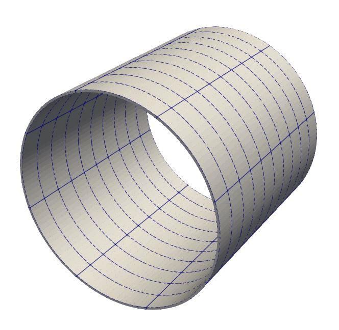
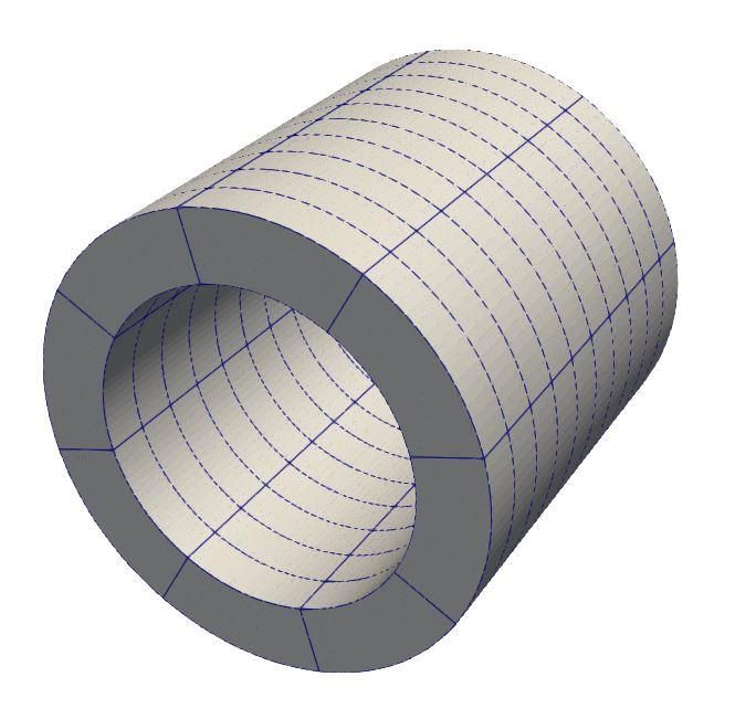
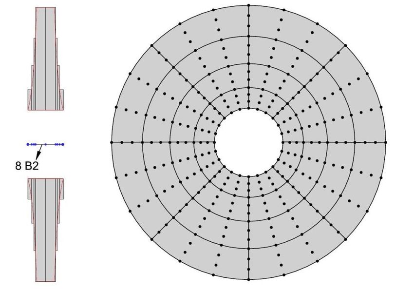
Alessandro Maturi - s255506 11

List of Figures

Chapter 1
  Fig. 1.1 Virus Lag, courtesy of LIMES – Rivista Italiana di Geopolitica [1] 17
  Fig. 1.2 Ticket Price Breakdown 18
  Fig. 1.3 Speed index for main shaft aircraft engine bearings. 19
  Fig. 1.4 Tacoma Narrows Bridge – 1940 – Washington State – USA 20
  Fig. 1.5 Single degree of freedom vibrational model (1 DOF) 20

Chapter 2
  Fig. 2.1 History of Rotordynamics 21
  Fig. 2.2 James Watt and its Steam Engine 22
  Fig. 2.3 Jeffcott Rotor 23
  Fig. 2.4 Wilfred Campbell and an example of his diagram 24
  Fig. 2.5 Oil-whip phenomenon 24
  Fig. 2.6 Chuck Yeager and the Bell X-1 25
  Fig. 2.7 Space Shuttle Main Engine (RS-25) and the powerful HPFTP 26

Chapter 3
  Fig. 3.1 Omega cross sectioned beam 31
  Fig. 3.2 L9 element in the natural coordinate system [10] 35
  Fig. 3.3 Stress-strain curve of a sample material 36
  Fig. 3.4 Geometrical Nonlinearity example =Buckling 37
  Fig. 3.5 Example of a 1D Lagrange Expansion FEM model 41
  Fig. 3.6 Assembly procedure for the 1D Lagrange Expansion FEM model 42

Chapter 4
  Fig. 4.1 Three-stringer spar 46
  Fig. 4.2 Natural modes in Paraview: mode 6 (17.67 Hz) and mode 10 (25.1 Hz) 46
  Fig. 4.3 First 15 natural frequencies (Hz) of the three-stringer spar [9] 47
  Fig. 4.4 Thin-walled cylinder 48
  Fig. 4.5 8 X 1 L16 Mesh 48
  Fig. 4.6 Thin-walled Cylinder Natural Frequency Chart [Hz] 49
  Fig. 4.7 Thin-walled Cylinder modes (ANSYS) 51
  Fig. 4.8 Thick-walled Cylinder Natural Frequency Chart [Hz] 53
  Fig. 4.9 Thick-walled Cylinder modes: Bending IV and Shell IV (Paraview) 53
  Fig. 4.10 Thick-walled Cylinder modes (ANSYS) 54

 Tesi di Laurea Magistrale – AA 2020-2021

12 Alessandro Maturi - s255506

  Fig. 4.11 Constant thickness disk mesh: (a) 1B3 along y-axis; (b) 2 X 16 L16 55
  Fig. 4.12 MUL2 mesh for the constant thickness disk 56
  Fig. 4.13 Mode 4 (91.7 Hz) and Mode 7 (115.5 Hz) in Paraview 56
  Fig. 4.14 1D-CUF model of the variable thickness disk, (1/2/3/4) × 8 L16 57
  Fig. 4.15 Mode comparison between ANSYS and Paraview (Disk) 57
  Fig. 4.16 Complex rotor Mesh schematization 58
  Fig. 4.17 Complex rotor Blueprint 58
  Fig. 4.18 Mode comparison between ANSYS and Paraview (Complex Rotor) 59
  Fig. 4.19 Bladed Disk Model 60
  Fig. 4.20 Bladed Disk modes (ANSYS & Paraview) 62

 Chapter 5
  Fig. 5.1 Realistic example of a Campbell diagram [15] 63
  Fig. 5.2 Waterfall plot: influence of the bilinear spring effect on vibrations [4] 64
  Fig. 5.3 Campbell Diagram for the constant thickness Disk 65
  Fig. 5.4 Campbell Diagram for the Variable thickness Disk 66
  Fig. 5.5 Thin walled Cylinder (Rotordynamic analysis) 67
  Fig. 5.6 Campbell Diagram for the Thin walled Cylinder 67
  Fig. 5.7 Thick walled Cylinder (Rotordynamic analysis) 68
  Fig. 5.8 Campbell Diagram for the Thick walled Cylinder 68
  Fig. 5.9 Shallow and Deep Shells 69
  Fig. 5.10 Campbell Diagram for the Shallow Shell 70
  Fig. 5.11 Campbell Diagram for the Deep Shell 70
  Fig. 5.12 Campbell Diagram for the Complex Rotor 71
  Fig. 5.13 Thin Ring Model 72
  Fig. 5.14 Campbell Diagram for the Thin Ring 72
  Fig. 5.15 Campbell Diagram for the Bladed Disk 73
  Fig. 5.16 3D solid FEM model for the analysis of Mistuning [16] 74
  Fig. 5.17 Mistuned Patterns analyzed for the Bladed Disk 75
  Fig. 5.18 Mistuned Bladed Disk – I blade Pattern - Campbell Diagram 75
  Fig. 5.19 Mistuned Bladed Disk – II blades Pattern - Campbell Diagram 76
  Fig. 5.20 Mistuned Bladed Disk – IV blades Pattern - Campbell Diagram 76

 Tesi di Laurea Magistrale – AA 2020-2021

Alessandro Maturi - s255506 13

List of Tables

Chapter 4
  Tab. 4.1 Free vibration analysis of the three-stringer longeron 47
  Tab. 4.2 Connectivity Matrix (Thin and Thick walled Cylinder) 49
  Tab. 4.3 Natural Frequency results for the Thin-walled Cylinder [Hz] 50
  Tab. 4.4 Natural Frequency results for the Thick-walled Cylinder [Hz] 52
  Tab. 4.5 Natural frequencies obtained for the Complex rotor [Hz] 59
  Tab. 4.6 Bladed Disk results in terms of natural frequencies [Hz] 61

 Tesi di Laurea Magistrale – AA 2020-2021

14 Alessandro Maturi - s255506

 Tesi di Laurea Magistrale – AA 2020-2021

Alessandro Maturi - s255506 15

 Part I
INTRODUCTION

Tesi di Laurea Magistrale – AA 2020-2021

16 Alessandro Maturi - s255506

 Tesi di Laurea Magistrale – AA 2020-2021

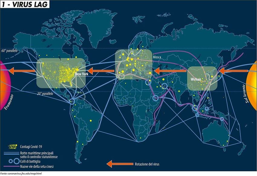
Alessandro Maturi - s255506 17

Chapter I
Reference framework
Air traffic has experienced a truly sudden development in recent decades. Indeed, the
International Air Transport Association (IATA) noted that between the 1970s and the late
1990s air traffic doubled in numbers approximately every 15 years, and it was expected that
this market would continue to grow annually at rates of 4% - 5% for next twenty years. These
forecasts inevitably had to collide with the heavy price of the COVID-19 pandemic, both in
terms of health and human lives, as well as in terms of the possibility of travel and movement
of the population.

The limitations on international connections, the more or less generalized "lockdowns" at a
global level (Fig. 1.1), the absence of tourism for almost the entire year of 2020 and a good
part of 2021, pending herd immunity acquired through vaccinations, resulted in a very violent
contraction of GDP in all nations and caused, among other things, serious financial problems
for the airlines. It is well known that this economic activity is one of the most difficult, as it
organizes and mobilizes some of the most complex systems that man has ever developed: first
of all it is based on aerospace engineering technology, which for regulations requires very
high standards of reliability and safety (1 ∙ 10−9 ); secondly, air traffic interfaces for the most
part with different nations and is therefore very susceptible to possible diplomatic incidents
and/or problems. Last but not least, air traffic is an activity that is highly dependent on the
market trend of some fixed expenses, among all the cost of fuel, which is by far the most
decisive.

 Figure 1.1 : Virus Lag, courtesy of LIMES – Rivista Italiana di Geopolitica [1]

 Tesi di Laurea Magistrale – AA 2020-2021

18 Alessandro Maturi - s255506

 If in a normal year the cash-flow margin of a standard airline is around 3% -5% of its revenue
 (Fig. 1.2), it is easy to understand how during these pandemic months many airlines suffered
 enormous financial losses or even bankruptcy, requiring and almost always obtaining state
 aid by virtue of the national interest.

 Figure 1.2 : Ticket Price Breakdown

 The ability to move people and goods, to connect different parts of the planet, but above all
 the ability of the aeronautical and aerospace sector to invest in technological research and
 innovation has always been recognized by nations with ambition for power, because it still
 represents one of the most advanced sectors of human activity. Despite this, the aeronautical
 field is always developing and is nowadays facing new challenges, among which the most
 relevant are certainly the attempt at an energy transition or at least the fight against global
 warming and the reduction of pollutant emissions and greenhouse gases.

 The needs of the final consumer (passenger) and these new environmental protection
 requirements for next generation aircraft translate into the study of new components of
 improved reliability and efficiency. Bearings and rotor systems are certainly two of the
 components that most significantly determine the reliability and effective mechanical
 performance of aerospace applications such as propulsion systems (turbine jet engines) and
 transmission systems (gearbox).
 These systems must withstand very severe and demanding operating conditions: the main
 shaft bearings of a modern aircraft engine experience very high levels of temperature and
 rotational speeds, while they must meet the highest safety and reliability standards trying to
 minimize weight. Such operating conditions and requirements represent an ongoing challenge
 to find improvements in all fields of rotor technology.

 Tesi di Laurea Magistrale – AA 2020-2021

Alessandro Maturi - s255506 19

The so-called “Bearing speed index”, that is the product of the bearing diameter and the
rotation speed, × represents a very useful parameter in providing information about the
centrifugal forces, the speed of the system and in general the operating conditions of the
rotor. Since there has always been the need to increase the specific thrust ("thrust-weigth-
ratio") and at the same time to reduce fuel consumption as much as possible, the rotation
speed of the shafts and the temperatures of the gases have constantly increased since when
jet engines were first introduced. Today, for example, the main shaft bearing operates at a
 
speed index of up to = 3.5 ∙ 106 .

To get an idea of the development of these components, it is possible to refer to this image
(Fig. 1.3) taken from reference [2], which presents the "speed index" trend of some
significant aircraft engines over the years.

 Figure 1.3 : Speed index for main shaft aircraft engine bearings. [2]

However, the more the speed index rises, the more problems related to rotor-dynamics begin
to arise: the higher rotational speeds produce greater centrifugal forces and the weight
limitation of the mechanical components and rotors lowers their stiffness, causing vibrations
which, if not checked, could lead to resonance and destruction of the machine.

Resonance describes the phenomenon of increased amplitude that occurs when the frequency
of a periodically applied force is equal or close to a natural frequency of the system on which
it acts. When an oscillating force is applied at a resonant frequency of a dynamic system, this
system will oscillate at a higher amplitude than when the same force is applied at other, non-
resonant frequencies, potentially reaching a critical level, beyond which the structure could
break.

This was the case with the Tacoma Narrows bridge, a suspension bridge built in 1940 in the
state of Washington on the Pacific coast. Problems related to vibrations immediately emerged

 Tesi di Laurea Magistrale – AA 2020-2021

20 Alessandro Maturi - s255506

 and became more visible especially during the particularly windy days, so much so that the
 population began to nickname him "Galloping Gertie (Fig 1.4).
 Unfortunately around ten o'clock on the morning of November 7, 1940, just over four months
 after its inauguration, the bridge began to sway and twist fearfully due to strong gusts of
 wind: about two hours later, following the showy twists of the central span which reached 70°
 of inclination, some tie rods broke, the structure reached the breaking point and the central
 span collapsed, falling into the water. This was the first evidence of that would be later called
 aero-elastic flatter, which is also related to resonance.

 Figure 1.4 : Tacoma Narrows Bridge – 1940 – Washington State - USA

 The simplest system we can think of dynamically is the undamped 1 degree of freedom (1
 DOF) system, which is shown in the next image (Fig 1.5). In this simple case, every physics
 book states that the resonant frequency (or natural frequency) is given by the following
 formula, where represents the oscillating mass, while represents the stiffness of the
 spring. Remember that we are considering an undamped system, so = 0.

 = √
 
 Figure 1.5 : Single degree of freedom vibrational model (1 DOF)

 It is therefore easy to understand how the reduction in stiffness can lower the resonance
 frequency to values that can be reached in today's rotating machines: Rotordynamics must be
 considered.

 Tesi di Laurea Magistrale – AA 2020-2021

Alessandro Maturi - s255506 21

Chapter II
History of Rotordynamics
“Human history may be built on the development of technology” J.S. Rao [3]

Although the invention of the wheel dates back to prehistoric times and the use of rotating
systems has accompanied humanity since the dawn of time, it was only during the 19th
century, thanks to the industrial revolution, that the first accurate studies on rotors were
conducted (Fig 2.1).
Only then, in fact, thanks to the invention of the steam engine and then the internal
combustion engine, it was possible to reach speeds that caused breakdowns to the rotating
machines, to the point of pushing scientists and engineers of that time to study the causes in
depth. As stated by J. Vance in his book [4] , “most rotordynamic investigations have been
motivated by machine problems or failures”.

 Figura 2.1 : History of Rotordynamics [5]

 Tesi di Laurea Magistrale – AA 2020-2021

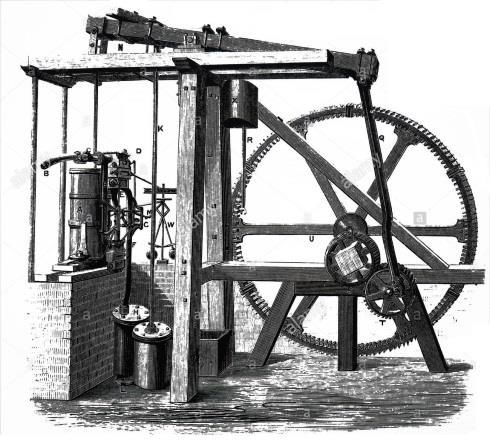
22 Alessandro Maturi - s255506

 The development of vibration theory, as a subdivision of mechanics, came as a natural result
 of the development of the basic sciences it draws from, mathematics and mechanics. The
 vibration phenomenon was identified already at Aeschylos times, and indeed Pythagoras of
 Samos (ca. 570-497 BC) conducted several vibration experiments with hammers, pipes and
 strings, of which he analyzed the harmonics. He was even able to prove with his experiments
 that natural frequencies are system properties and do not depend at all on the magnitude of
 the excitation. This proves that in the ancient world there was some kind of progress about
 vibration theory and a basic understanding of the principles of natural frequency, vibration
 isolation and their measurements. However, this original body of knowledge had very limited
 use in engineering and innovation, due to the low level of production technology and
 machinery speeds, as well as a substantial lack in all the other subjects involved.

 For example, calculus and mechanics, which are the basis for the analytical treatment of the
 problem, began to be developed only during the 1600s and 1700s, with the discoveries of
 Galileo, Newton and Leibniz. The early stages of mechanization and the first industrial
 revolution, together with the utilization of chemical energy with the associated high-power
 machinery (Fig 2.2), introduced numerous vibration problems, and the rapid development of
 calculus and continuous mechanics led to rapid development of the vibration theories by the
 mid-19th century.

 Figura 2.2 : James Watt and its Steam Engine

 The wave equation was first introduced by D’Alambert in a memoir to the Berlin Academy in
 1750 and the solution of the string equation is due to Daniel Bernoulli. The first mathematical
 solution to the problem of the vibrating string was obtained by Lagrange in 1759, considering
 it as sequence of small masses: an approach still used today. Euler and James Bernoulli tried
 to solve the vibrating plate and shell problem analytically, obtaining the differential equations
 considering them as consisting of two system of beams perpendicular to each other. Further
 major improvement was made by Poisson and Kirchhoff, but it was eventually Navier who
 gave a rigorous theory describing the bending vibrations of plates.

 This was meant to be just a fast recap of some of the major development in the sciences that
 are at the base of rotordynamics. There are countless other scientists and scholars worthy of
 having made great developments in this field, but to list them all would have been impossible
 in these few pages.

 Tesi di Laurea Magistrale – AA 2020-2021

Alessandro Maturi - s255506 23

Rotating machines began to be manufactured in what we can call mass production
concurrently with the development of waterwheels for hydraulic power in the early 1800s
and steam turbines in the late 1800s. One of the first dynamic problems which was
encountered was the critical speed: in this situation, a vibration caused by the rotor imbalance
is amplified by the resonance with the natural frequency of the system, causing the rotor axis
to deflect.

Research on rotordynamics spans at least a 140-year period, starting with Rankine’s paper
about the whirling motions of a rotor, which dated back to 1869. The famous Scottish
engineer and physicist discussed the relationship between centrifugal forces and restoring
forces, concluding that any kind of operations above a certain rotational speed would be
impossible to achieve.

Much progress in this area was achieved by the end of the nineteenth century, mainly thanks
to the contribution of De Laval and Stodola. The first was a Swedish engineer who invented a
one-stage steam turbine and succeeded in its operation, first with a rigid and then with a
flexible rotor. His greatest achievement was to show that it was possible to operate in
supercritical field by operating at a rotational speed which was about seven times larger than
the critical speed, as can be gleaned from Stodola's 1924 publication [6]. He was the first to
notice that he could accelerate through the critical speed, and that the operation at
supercritical speeds, way above the critical one, was very smooth.

In 1916 Stodola introduced for the first time the concept of bearing damping in
rotordynamics, proving that the presence of damping limits the amplitude due to the
unbalance at the critical speed. He also observed the decrease of the critical speed due to
damping and was able to compute the phase angle with bearing damping.

As we can imagine, in the early days the major
concerns for researchers and designers was to try
to predict the value of the critical speed, because
their major concern in designing rotating
machinery was to avoid resonance.

The first recorder fundamental theory of
rotordynamics can be found in a scientific paper
published by Jeffcott in 1919: because of his study
 Figure 2.3 : Jeffcott Rotor
and theory, we now call Jeffcott Rotor the system
consisting of a shaft with a disk positioned at its
midspan (Fig 2.3).
He obtained a correct analysis of the critical speed inversion with damping included, and, as a
consequence, the predominant design philosophy changed and accepted the practice of
turbomachinery supercritical operations. During the same years, also the dynamics of elastic
shafts with disks, the dynamics of continuous rotors and the balancing of rigid rotors were
analyzed, alongside with the approximate determination of critical speeds of rotors with
variable cross sections.

 Tesi di Laurea Magistrale – AA 2020-2021

24 Alessandro Maturi - s255506

 Thereafter, the center of research and scientific world shifted from Europe, that was emerging
 from the tragedy of the First World War, to the United States , and the scope of rotordynamics
 expanded to consider many other phenomena. Wilfred Campbell investigated the vibrations
 in steam turbines in detail, while working at General Electric in the 1920s: he came up with
 the idea of plotting a diagram, representing critical speed in relation to the cross points of
 natural frequency curves and the straight lines proportional to the rotational speed. This
 concept is now widely used and we call it Campbell diagram, after the name of his developer
 (Fig 2.4).

 Figure 2.4 : Wilfred Campbell and an example of his diagram

 As the rotational speed increases above the first critical speed, the occurrence of self-excited
 vibration became a serious problem. Newkirk and Kimball recognized the phenomenon
 according to which the internal friction of shaft materials could cause an unstable whirling
 motion: they investigated a whirl instability called oil whip, caused by the oil film in the small
 clearance of journal bearings (Fig 2.5) which occurs at about two times the critical speed [7].

 Figure 2.5 : Oil-whip phenomenon

 Rotor instability due to thermal strains caused by rubbing was observed by Newkirk in 1926:
 he spotted a forward whirl induced by a hot spot on the rotor surface, generated in the same
 point where contact between the rotor and the surroundings happens. This hot-spot
 instability is therefore called Newkirk effect.

 Tesi di Laurea Magistrale – AA 2020-2021

Alessandro Maturi - s255506 25

During and after the 2nd World War there was a rapid progress in increasing the size and the
power density of turbomachinery, in search of technological supremacy and for issues related
to the more developed arms race, especially in military aviation.
The theory that explains most fundamental rotordynamics problems had been already
published by this time, but the new sophisticated applications brought new and complex
challenges in using these theorems to produce practical design analysis.

As an example, the arrival of high-speed rotating machines made it necessary to develop a
balancing technique for flexible rotors. In 1945 Prohl published a new method for calculating
critical speeds of flexible rotors with many “stations”, consisting of wheels or lumped masses
along the rotor shaft. His method is now known as Transfer Matrix method. Moreover, up until
the fourth decade of the 20th century, most analytical models of critical speeds and whirling
eigenvalues had neglected gyroscopic effects of the spinning wheels. With the low-speed
machines of the past, the errors in results were generally small and negligible, but now the
continuous growth of turbomachinery operating speed requested that the gyroscopic effects
to be taken into account. This breakthrough was accomplished by Greene in 1948.

After Frank Whittle and Hans von Ohain developed the jet engine independently of each other,
the study of rotordynamics gained even greater momentum, in the search for the
development of an engine capable of pushing an aircraft beyond the sound barrier. Success
was finally achieved in 1947, when Chuck Yeager pushed his Bell X-1 past Mach 1 over the
desert areas of California (Fig 2.6).

 Figure 2.6 : Chuck Yeager and the Bell X-1

In the 1950s it was found that sub-synchronous whirling in steam turbines was somehow
related to the steam force on the turbine wheels: a thorough investigation performed by
Thomas in Germany showed that a variation of tip clearance around the blades could create a
resultant follower force on the whirl orbit, which can unbalance the rotor. This particular kind
of instability in steam turbines became known as steam whirl.

The design requirements for speed and specific power of turbomachinery equipment have
been rapidly increasing since the 1960s, coinciding with the space rush and the race to the
moon.

 Tesi di Laurea Magistrale – AA 2020-2021

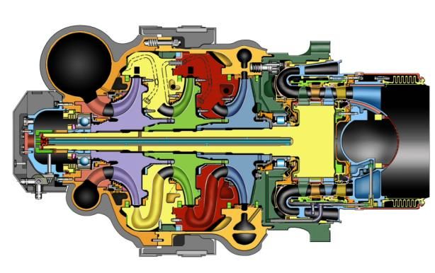
26 Alessandro Maturi - s255506

 A striking example is the rocket engine turbopumps: the Space Shuttle Main Engine High
 Pressure Fuel Turbo-Pump (SSME HPFTP) reached speeds of over 35.000 rpm [8], driven by
 70.000-hp turbines about the size of a frisbee (Fig 2.7).

 Figure 2.7 : Space Shuttle Main Engine (RS-25) and the powerful HPFTP

 These kind of performance result in machines that are likely and easily to be unstable in sub-
 synchronous whirl. Designing multiple stages on one single shaft result in long, flexible shafts
 with accentuated bending modes, which makes difficult the suppression of any instability.
 Because these machines must always be lightweight, the rotors are consequently even more
 flexible, making balancing more difficult.
 The presence of many stages on one shaft produce multiple critical speeds, which in theory
 can be balanced by having a number of balance planes which is identical to the number of
 critical speed traversed. In practice, however, is often difficult to realize a large number of
 balance planes, so some methods have been developed to achieve excellent results with fewer
 of these planes. The most popular is the least-square balancing method published by Goodman
 at General Electric in 1964, as an extension of the influent coefficient method, developed
 only a few years earlier in the US thanks to the progress of the computers.

 In the latter half of the last century, various vibrations due to fluid were studied, but these
 arguments are well beyond the scope of this work. A more recently developed topic is the
 study of the non-linear field.

 As rotors became lighter and their operational speeds continue to grow higher, the
 occurrence of nonlinear resonances became a serious problem. Yamamoto studied various
 kinds of nonlinear resonances after reported on subharmonic resonances due to ball bearings
 in 1955. He also discussed systems with weak nonlinearity that can be expressed by a power
 series of low order. In general, it turned out that the most frequent cause of strong
 nonlinearity in aircraft gas turbines is the radial clearance of squeeze-film damper bearings.

 Much more recent is the study of rotordynamics in the non-linear deformation field of the
 material, which can deform beyond its elastic range given the enormous forces and stresses
 involved in today’s turbomachinery.

 Tesi di Laurea Magistrale – AA 2020-2021

Alessandro Maturi - s255506 27

This thesis work will be carried out in this precise context, exploiting the potential of the finite
element method to perform the calculations of natural frequencies.

During the practical design of rotating machinery it is in fact compulsory to know accurately
the values of the natural frequencies, modes, and forced responses to unbalances in complex-
shaped rotor systems. The representative techniques used for this purpose are the transfer
matrix method and, nowadays, the finite-element method.

The latter was first developed in structural dynamics and then used in almost all fields of
modern engineering: the very first application of this method to a rotordynamic problem, a
rotor system in particular, was made by Ruhl and Booker in 1972. Since then, the use of FEM
in rotordynamics has taken off, and it was generalized by considering rotating inertia,
gyroscopic moment and axial forces.

In this chapter, we have tried to briefly summarize the history of rotordynamics: from
antiquity, passing through the Renaissance, the industrial revolution, wars and until today,
numerous other pages still remain to be written in this exciting field of engineering.

 Tesi di Laurea Magistrale – AA 2020-2021

28 Alessandro Maturi - s255506

 Tesi di Laurea Magistrale – AA 2020-2021

Alessandro Maturi - s255506 29

 Part II
UNIFIED FORMULATION THEORY

 Tesi di Laurea Magistrale – AA 2020-2021

30 Alessandro Maturi - s255506

 Tesi di Laurea Magistrale – AA 2020-2021

Alessandro Maturi - s255506 31

Chapter III
Theoretical References and CUF
We now consider a beam structure with an
Ω cross section which lays on the plane
of a Cartesian reference system (Fig 3.1). As
a consequence, for the right-hand-rule, the
beam axis is placed along the Cartesian 
and it measures [11].

The transposed displacement vector is
therefore given by the following expression:

 ( , , ) = { } 
 Figure 3.1 : Omega cross sectioned beam
where are the displacement
components along the 3 main directions.

The stress, , and engineering strain, , components are expressed in vectorial form in the
same way, with no loss of generality:

 = { } 

 = { } 

In this thesis project, linear elastic metallic beam structures will considered initially. Hence,
the Hooke’s law provides these constitutive relations:

 = 
The characters used in this formula are deliberately in bold and not in italics, to indicate the
operation between vectors, where the material matrix is given by the following:

 11 12 13 0 0 0
 12 22 23 0 0 0
 23 33 0 0 0
 = 13
 0 0 0 44 0 0
 0 0 0 0 55 0
 [ 0 0 0 0 0 66 ]

 Tesi di Laurea Magistrale – AA 2020-2021

32 Alessandro Maturi - s255506

 The coefficients of the stiffness matrix depend only on the Young modulus and the Poisson
 ratio , in these forms:
 (1 − ) 
 11 = 22 = 33 =
 (1 + )(1 − )
 
 12 = 13 = 23 =
 (1 + )(1 − )
 
 44 = 55 = 66 =
 2(1 + )

 As far as the geometrical relations are concerned, the Green-Lagrange nonlinear strain
 components are considered. For this reason, the displacement-strain relations are expressed
 as:
 = + = ( + ) 
 where clearly the and subscripts stand for “linear” and “non-linear”, so and are
 the linear and nonlinear differential operators, respectively. For the sake of completeness,
 these differential matrix operators are given below:

 1 1 1
 0 0 ( )2 ( )2 ( )2
 2 2 2
 0 0 1
 ( )
 2 1
 ( )
 2 1
 ( )
 2
 2 2 2
 0 0 1 1 1
 = = ( )2 ( )2 ( )2
 0 2 2 2
 
 0 
 
 [ 0] [ ]

 (.) (.) (.)
 Obviously, the notation used is that = = =
 
 Matrix and are also used to define the equilibrium conditions and equations, which
 can be written in vectorial form invoking a loading vector :

 ( + ) = = = { }

 Mechanical boundary conditions must be fulfilled on which represents the portion of the
 body surface where the mechanical conditions on the loading are given, with normal 
 vector.
 + + = 
 { + + = 
 + + = 

 In this formula = { } is the applied loading vector per unit area on the
 aforementioned surface .

 Tesi di Laurea Magistrale – AA 2020-2021

Alessandro Maturi - s255506 33

As stated in reference [9], the mechanical and geometrical boundary conditions must be fully
defined to complete the set of equations related to the displacement formulation of the 3D
problems: these can be obtained by merging Hooke’s Law and the strain-displacement
relation, obtaining a vectorial formula which represents the boundary-value problem of the
3D elasticity problem, whose solution then leads to the calculation of the deformed
configuration, as well as the calculation of the unknown displacements .

This equation of elasticity and the related displacement approach can conveniently be
formulated by means of the PVW (Principle of Virtual Work) or the PVD (Principle of Virtual
Displacement). This variational approach is a very powerful and effective method, which can
deal with weak forms and the derivation of Finite-Element (FE) matrices, easily processable
by a calculator.

Some multi-dimensional models of aerospace rotordynamic-related structures will be
developed using the formalism from the Carrera Unified Formulation (CUF) [9]. The CUF
provides one-dimensional (beam) and two-dimensional (plates and shells) theories that can
extend well beyond the classical theories (Euler, Kirchhoff, Reissner, Mindlin), exploiting a
condensed notation. The latter works by expressing the displacement fields in
correspondence of the cross section (when we consider a beam) and along the thickness (in
the case of plate and shell) in terms of basic functions, whose forms and orders are arbitrary
and can be chosen by the user itself. The use of a unified notation leads to the definition of the
so-called fundamental nucleus (FN) of all the matrices and FEM vectors involved.

The FNs consist of just a few mathematical statements, whose forms are totally independent
from the theory of structures (TOS) employed. The FNs derive from the 3D elasticity
equations by the application of the principle of virtual displacements (PVD) and can be easily
obtained for many cases, in every number of dimensions considered (1D, 2D or 3D).

Generally, the 1D and 2D Finite-Elements obtained with the CUF present some advanced
functionalities, as they are able to achieve results which are usually provided only by 3D
elements, but with a much higher computational costs. Moreover, the 1D elements are
particularly advantageous as they can deal with 2D and 3D problems in a proper and exact
way.

In this master thesis work the 1D elements will be mostly utilized, since the various structures
which will be analyzed can be effectively studied using a combination of these simple
elements.

The CUF can be defined as a hierarchical formulation, which considers the order of the theory
as an input of the analysis: it enables one, at least theoretically, to derive an infinite number of
sophisticated displacement models [10]. This particularity makes it able to deal with a wide
variety of structural problems without the need to introduce specifically designed
formulations for each one of them, and right here lies the powerful potential of this theory.

The so-called non-classical effects, such as warping, planar deformations, shear effects,
flexural-torsional coupling, are taken in consideration simply increasing the order of the
theory in an appropriate manner.

 Tesi di Laurea Magistrale – AA 2020-2021

34 Alessandro Maturi - s255506

 In the first stages of its development, the CUF theory was founded on the use of Taylor-like
 polynomials to define the range of displacements on the beam cross-section. Static analyzes
 carried out in the past showed the effectiveness of the theory when dealing with warping
 phenomena, deformations in the plane and when dealing with effects due to the Shear loading.

 Taylor Expansion (TE) models proved to be very efficient when considering prismatic
 structures, but they also showed some limitations when the rotor components presented
 different deformability. For this reason the use of Taylor polynomials has some intrinsic
 limitations, mainly due to the fact that the terms of the expansion of the displacement range
 do not have always a physical meaning.

 In order to overcome these problems it has recently been implemented a new beam theory,
 which describe the displacement field of the cross section with Lagrange-like polynomials.
 The choice of these kind of expansions leads us to have only variables of displacements. The
 component-wise (CW) approach has therefore been extended, within the CUF framework, to
 the rotordynamics problem, and Lagrange-like polynomial expansions have been adopted to
 develop the refined displacement theories.

 The choice of Lagrange polynomials, besides bringing numerous benefits in terms of
 versatility of the structural models, allows the user to find even more accurate results than
 Taylor's expansion-based polynomials models. This permits us to consider many phenomena
 that otherwise would only be identifiable via 2D or 3D models, with their higher time-
 consuming and computational cost. In addition, the LE elements allows us to model each
 structural component of the rotor with an arbitrary degree of accuracy [10], giving us the
 chance to focus the analysis in pre-established areas, where we think the core of the problem
 lies and where we can adopt some localized mesh refinements.

 Derivation of solid beam finite elements by Carrera unified formulation
 In the 1D-CUF framework, the tridimensional displacement field u( , , , ) = ( , , ) is
 approximated with an expansion of generic cross-sectional functions which allow us to
 isolate the effect of the axial coordinate to the shape functions only:

 3 : u( , , , ) = u ( ) ∙ ( , , ) ∙ 1 = 1 … 3 

 1 : u( , , , ) = u ( ) ∙ ( ) ∙ ( , ) = 1 … 1 ; = 1… 

 is the 1D shape function, u is the vector of the generalized displacements, represents
 the number of terms of the expansion, which is an input by the user, and the index refers to
 the FE discretization, varying from 1 to the maximum number of nodes in the finite-element.
 In accordance with the generalized Einstein’s notation, indicates summation, while the
 ( , ) are the cross-sectional Lagrange polynomials used to deal with the arbitrary shape
 geometry. As mentioned before, even if we can use every type of functions, the connection
 between the elements becomes very simple when we use Lagrange-type expansions.

 Tesi di Laurea Magistrale – AA 2020-2021

Alessandro Maturi - s255506 35

In this case, the beam kinematics is obtained as a combination of Lagrange polynomials, which
are defined within sub-regions (or elements) delimited by an arbitrary number of points. This
number of points determines the order of the polynomial. For the nine-point element L9
shown in the figure below (Fig 3.2) the interpolation functions are the following:

 Figure 3.2 : L9 element in the natural coordinate system [10]

 1 2
 = ( + )( 2 + ) = 1,3,5,7
 4
 1 2 2 1
 = ( − )(1 − 2 ) + 2 ( 2 − )(1 − 2 ) = 2,4,6,8
 2 2
 = (1 − 2 )(1 − 2 ) =9

Here, and vary from −1 to +1, whereas and are the coordinates of the nine
points of the element, whose locations in the natural coordinate frame are shown in Fig 3.2.
As a consequence, the displacement field of the L9 element is:

 = 1 1 + 2 2 + 3 3 + ⋯ + 9 9
 = 1 1 + 2 2 + 3 3 + ⋯ + 9 9
 = 1 1 + 2 2 + 3 3 + ⋯ + 9 9

In these equations all the unknowns ( 1 , … , 9 ) have the same dimension: they are the
displacement variables of the problem and represent the translational displacement of each of
the nine points used to define the L9 element of the cross-section. these formulas can now be
used to derive the expressions of the normal and tangential strains and stresses: together
with Hooke's Law and the application of the classical finite element technique, this leads to
the following expression for the generalized ( ) and nodal ( ) displacement vector.

 ( , ) = ( ) ( ) ( ) = { 
 
 } 
 . 

 Tesi di Laurea Magistrale – AA 2020-2021

36 Alessandro Maturi - s255506

 At this point, it should be underlined that the choice of the cross-section polynomials sets for
 the Lagrange-Expansion kinematics is completely independent of the choice of the beam finite
 element to be used along the beam axis.

 This means that the selection of the type, the number and the distribution of cross-sectional
 polynomials does not affect the discretization along the axis: the 1D CW approach has in
 fact allowed us to greatly simplify the problem, as we can choose whatever elements we find
 appropriate to describe the kinematics in this axial direction. In this thesis work classical 1D
 finite elements with four nodes (B4) are adopted, so a cubic approximation along the -axis is
 generally assumed.

 Geometrically Nonlinear analysis of a structure
 Structural analyses are commonly carried out in the linear elastic field, where the following
 hypothesis are assumed:
  the material is elastic-linear, and its mechanical properties are invariable with respect
 to the level of stress applied to the structure;
  the equilibrium equations are formulated in the undeformed configuration or, in the
 case of structures subject to a state of pre-stress, in an initial reference state;
  the deformations to which the structure is subjected are considered “small” and do not
 significantly influence the structural response.
 These hypotheses allow considerable and very often valid simplifications in the structural
 analysis, while the removal of one or more of them leads to the introduction of elements of
 non-linearity in the analysis. In general, a structural analysis can take into account two types
 of non-linearity.
 The first one is the physical non-linearity of the material, which arises when it presents a non-
 linear constitutive bond, entering the plastic field once the elastic limit has been exceeded.
 This effect can be seen on the stress-strain curve (Fig 3.3) for a specific material, that gives the
 relationship which holds between the stress applied to it and the strain with it responds.

 Figure 3.3 : Stress-strain curve of a sample material

 Tesi di Laurea Magistrale – AA 2020-2021

Alessandro Maturi - s255506 37

These diagram is obtained by gradually applying a load to a test coupon and measuring the
deformation: from this two data the stress and strain can be determined and plotted on a
graph as a curve, which reveal many of the properties of the material, such as the Young’s
modulus, the yield strength and the ultimate tensile strength.

The second typology of non-linear effects are those that will be treated in this thesis, namely
geometric non-linearity. The before mentioned hypothesis of small displacements is here
abandoned, as first order deformations produce a non-negligible displacement of the load
application point. It follows that the stresses and displacements of the model need to be
recalculated considering the loads applied to the deformed configuration and following an
iterative procedure. This phenomenology can occur in the following cases:

  in presence of large displacements, when there is a big difference between the
 undeformed and the deformed configuration of the structure;
  when the so-called follower forces arises and the deformation changes the direction of
 the load with respect to the undeformed configuration;
  In general, the stress-state of the structure always
 introduces a side effect, which can be defined as stress
 stiffening or stress softening. For example, from
 previous studies we know that the rotation and the
 consequent centrifugal forces that derive from it tend
 to stiffen the structure, increasing the value of the
 natural frequencies.
 We therefore expect to find this trend in the analysis
 of the Campbell diagrams that will be carried out in
 the following chapters. On the other hand, stress
 softening can manifest itself, for example, with elastic
 instability and buckling (Fig 3.4) produced by the Figure 3.4 : Geometrical Nonlinearity
 compression-state. example =Buckling

In most cases, the structural analyses are limited to the study of small displacement field.
However, today's engineering applications, especially in rotor components, have reached
rotational speeds and applied forces so high that they can deform the structure substantially,
radically changing its dynamic properties.

A geometrically non-linear FEM analysis allows us to consider the increase or reduction in
stiffness due to the stress-state related to large displacement, and it is therefore very
important to have suitable tools to analyze this situation as well, as it implies a much more in-
depth and complex mathematical treatment.

This type of analysis leads to results that are strictly dependent on the basic hypotheses from
which we started and consequently it will be necessary to pay particular attention to their
validation: as we said, the geometrically non-linear analysis provides looser assumptions only
regarding the deformations magnitude, while it predicts that the material always remains in
the linear-elastic range, where the stress-strain graph takes the form of a straight line.

 Tesi di Laurea Magistrale – AA 2020-2021

38 Alessandro Maturi - s255506

 Nonlinear Governing Equations of Vibrating Structures
 Consider now an elastic system which is in equilibrium under a set of applied forces and some
 prescribed geometrical constraints. The principle of virtual work (PVW) establishes the well-
 known equilibrium condition between the virtual variations of works done by the
 deformations , inertia and external forces . In particular, the PVW states
 that [12]:
 = + . 

 In this case, the strain energy is defined as the body volume integral of the virtual strains
 multiplied by the stress vector, according to the following formulation:

 = ⟨ ⟩ ℎ ⟨(… )⟩ = ∫ (… ) 
 
 If we apply the hypothesis of small deformations, using the Green-Lagrange nonlinear strain
 components already mentioned in the previous pages the displacement-strain relation
 becomes
 = ε + ε = (b + b ) = ( 
 + ) 

 While the 3D constitutive equation is still given by the well-known Hooke’s Law formula:

 = 

 In this case, 
 and are the linear and nonlinear matrices obtained within the CUF finite
 element method framework as described above, while is the 6 × 6 matrix of linear elastic
 material coefficients. Substituting these equations into the . 2 and using the and indexes
 for the terms related to the virtual variation, we obtain that:

 = ⟨ ⟩ = ⟨( + 2 ) ( 
 + )⟩ 
 
 = 0 + + + . 
 
 = 

 In this last equation several K matrices appear, which will now be analyzed in detail: the
 
 secant stiffness matrix includes the linear terms 0 , the two first-order nonlinear
 
 contributions and , and the second-order nonlinear matrix, given by . These
 are 3 × 3 arrays, called Fundamental nuclei (FN) and their expressions are not affected by the
 type or the number of functions which we decided to use for the kinematic expansion. As a
 consequence, every type of beam theories can be automatically implemented by exploiting the
 indicial notation of this unified formulation.

 Tesi di Laurea Magistrale – AA 2020-2021

Alessandro Maturi - s255506 39

If we are looking for a non-linear solution, we must necessarily identify the equilibrium point
reached by the structure, and then consider the oscillations around this point. In fact, similarly
to that of the internal forces, the virtual work done by the inertial forces is defined as the
body volume of the small perturbations vector around a steady nonlinear equilibrium
position ̂ = [ 
 ̂ ̂ ̂ ] , multiplied by the expression of the inertial forces itself:

 ̂ ⟩ = ∫ ( 
 = ⟨ ̂ ) . 
 
All these terms are expressed with respect to a coordinate reference frame attached to the
rotor that rotates at constant speed Ω about its -axis. According to that, the inertial forces are
given by:

 ̂ ̈
 − ̂ ̇ 
 ̂ 
 ̈ 2 2
 ̂ ) − 2 Ω ( 0 ) + Ω ( 0 ) + Ω ( 0 )
 = − ( . 
 ̂ ̇
 
 ̂ 
 ̂ ̈
 
Combining and merging . 1, 4 and 5 the FN of the mass matrix is readily obtained, as
 
well as the Coriolis matrix , the centrifugal matrix and the vector of centrifugal
 
forces .

We now have all the ingredients needed to carry out our goal: the non-linear analysis. If any
 
external loads ext are applied to the structure, the nonlinear equation to be solved becomes:

 = + Ω

However, this formulation is still too complex to be solved analytically, as we explained how
the matrix still contains all the non-linear terms: the solution needs to be determined
through a Newton-Raphson incremental scheme, which requires the linearization of . 3:

 ( ) = ⟨ ⟩ + ⟨ ( ) ⟩
 
 = ( 0 + 1 + ) . 
 
 = 

Here we introduced the tangent stiffness matrix, , whose fundamental nucleus includes
the before mentioned nonlinear contribution of the Hooke’s law, the linear stiffness matrix
 
 0 and the geometric stiffness matrix .

 Tesi di Laurea Magistrale – AA 2020-2021

40 Alessandro Maturi - s255506

 The analysis of this thesis is aimed at the calculation of the natural frequencies of some
 structural models. These natural frequencies and mode shapes ̅ associated with small-
 amplitude vibrations are significantly affected by the equilibrium point they oscillate about,
 and can be obtained assuming a harmonic solution for the following dynamic equation:

 ̂̈ + 
 ̂̇ + ( ( e ) + ) 
 ̂= ̅ 
 ̂= 
 . 

 This formulation holds for large displacements and large rotations of the structure until
 reaching its equilibrium state, around which only small vibrations are allowed.

 In the following chapters comparative analyses between non-linear theory and linearized
 theory will often be carried out. In fact, in order to reduce the computational effort and the
 mathematical complexity, this last . 7 can be linearized, considering only the linear part of
 the geometric stiffness matrix .

 = 0 + 1 + 
 ≈ 0 + ∗ 

 This new geometric stiffness matrix ∗ derives from the geometric strain energy, obtained by
 the product between the nonlinear component of strains and the initial stress vector 0 .
 The computation of the rotation-induced stresses is performed by a static linear analysis in
 which the rotation force Ω appears.

 ( 0 + Ω )|Ω=1 
 ̂ = Ω |Ω=1

 It is important to specify that the newly obtained ∗ matrix differs from the previous one
 ( ) because in this particular case the stress field is computed only considering the linear
 part of the strain field, since the problem is being linearized. The dynamic system therefore
 becomes linearized, which means that it is analytically solvable, and requires much less
 computational effort:

 ̂̈ + 
 ̂̇ + ( 0 + Ω2 ∗ + ) 
 ̂= ̅ 
 ̂= 
 . 

 Tesi di Laurea Magistrale – AA 2020-2021

Alessandro Maturi - s255506 41

The Assembly Procedure
The structural configuration of Fig 3.5 is now used to explain the assembly procedure of the
various matrix involved in the previous dynamic systems. Theoretically speaking, a prismatic
structure can be modeled with beam or solid elements: in this example one Lagrange element
with 4 nodes (L4) is used on the cross-section, while 2 beam elements with two nodes are
used to model our structures along its longitudinal axis. The image shows that the every beam
model has four nodes in each transversal section. The unknown displacements are, therefore,
given by:

 = ( ) = 1,2,3,4 = 1,2,3,4

 Figure 3.5 : Example of a 1D Lagrange Expansion FEM model

Otherwise, we also could have modeled the structure with a generic number of 3D elements,
with 8 nodes each. The latter is usually the strategy of commercial FEM codes, which
automatically generate a very dense mesh with a huge number of elements, that
determines an increase in the computational cost.

For this reason, now we want to focus on the numerical procedure that allows us to derive
and assemble the stiffness and mass matrices of the entire structure, starting from the 1D and
Lagrange elements, that will be used in the course of this thesis.

As both beam models have the same unknowns, the imposition of the compatibility condition
between shared nodes is very simple, considering that nodes 2 and 4 coincides in the final
assembled model:

 21 = 41 22 = 42 23 = 43 24 = 44

 Tesi di Laurea Magistrale – AA 2020-2021